The Simplex Algorithm whose invention is due to George Dantzig in 1947 and in 1975 it earned him the National Medal of Science is the main method for solving linear programming problems.

|
|
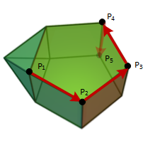
The simplex algorithm performs iterations within the extreme points set of feasible polytope region, checking for each one if a optimality criterion holds.
|
Given a linnear programming standard problem P:
Minimize \( C^t x \)
Subject to
\( \begin{matrix} Ax=b \\ x\geqslant 0 \end{matrix} \).
Where
\( A \in \mathbb M _{mxn}, \, rnk(A)=m ,\,\, b \in R^{m}, \, C \in R^{n}, \,\, n \geqslant m \).
Where m is the number of constraits or rows of matrix A, also dimension of vector b, and n is the number of variables (columns of matriz A or dimension of vector C).
If the problem P has optimal solution x
k finite, we know from the
Linear Programming Theory that such x
k
belongs to the
extreme points set of the feasible region S.
The Simplex Algorithm basic idea is to perform iterations over the extreme points set until a condition called
optimality criterion holds.
If is holds at a certain extreme point x
k, then this is the solution for P.
Let suppose that x is an
extreme point of S. Because of the extreme points set is conformed by solutions of an Bx=b with B submatrix of intial A, x can be write as
\( x=\begin{bmatrix} B^{-1}b \\ 0\end{bmatrix} \).
with B as said a mxm-square A submatrix with rank m.
We can decompose A into B and N submatrices as follows:
\( A=\begin{bmatrix} B \\ N\end{bmatrix} \)
Again: B is a mxm submatrix with rank m corresponding to solution of system Bx=b. And N is the matrix formed with the remaining columns from A.(Remember that n≥m).
Lets w another point from the feasible region S. Then
Aw = b, ie
\(Bw_{B} + Nw_{N} = b \).
Because B is invertible
\(w_{B} = B^{-1}b - B^{-1}Nw_{N} \)
Applying C
t to w we obtain
\( C^{t}w = C_{B}^{t}w_{B} + C_{N}^{t}w_{N} \)\( = C_{B}^{t}(B^{-1}b - B^{-1}Nw_{N}) + C_{N}^{t}w_{N} \)\( = C_B^tx_B + C_{N}^{t}w_{N} - C^tB^{-1}Nw_{N} \)
Because w belongs to feasible region, we know that
w
N ≥ 0, so if x were the optimal solution then it must holds:
\((1) \,\,\,\,\,\,\,\,\,\,\,\,\,\,\,\,C_{N}^{t}-C^t_{B}B^{-1}N\, \geq \, 0\).
This is the basic idea from the Simplex Algorithm that we were talking before, and it is call
Optimality Criterion
The Simplex Algorithm Optimality Criterion
$$ C_{N}^{t}-C^t_{B}B^{-1}N\, \geq\, 0 $$
If this condition holds, then x is the optimal solution of P.
The Optimallity Criterion equation has as coordinates
\(c_{j} - C^t_{B}B^{-1}a_{j} = c_{j} - X_{B}a_{j} = c_{j} - z_{j} \)
Being a
j, column vector of N.
This allows us to sum up the optimality criteria as follows:
$$ c_{j} - z_{j} \geq 0 $$
Let us suposse now than (1) does not holds, thus we have
\( C_{N}^{t}-C_{B}B^{-1}N\, < 0 \)
Then there are two possible cases:
Case 1
\( y_{j} = B^{-1}a_{j} \leqslant 0, \; \forall j \) then we can build
\( x= w+\lambda d_{j} \) siendo \( d_{j}=\begin{bmatrix} -B^{-1}a_{j} \\ e_{j} \end{bmatrix} \)
we know that d
j is an extreme direction of feasible set S, in particular
\( Ad_{j} = 0 \)
so \( x= w+\lambda d_{j} \) is also feasible solution \( \forall \lambda d_{j} \geqslant 0 \)
On the other side:
\( C^{t}x = C^{t} (w+\lambda d_{j} ) = \)\( C^{t}w + \lambda(-C^{t}B^{-1}a_{j})d_{j} = \)\( C^{t}w - \lambda(z_{j}-c_{j}) \mapsto - \infty \) when \( \lambda \mapsto \infty \)
This means that we can build any solution as small as we want without leaving the feasible set S and so this is a
Unbounded case solution
Case 2
The vector\( y_{j} \) has at least one positive component
We determine the index s that meets
$$ s = min \{ k: \,\ c_{k} - z_{k} < 0 \} $$.
That is take the minimum of negative in \( c_{k} - z_{k} \).
Then it is possible to build any other feasible solution wich is within the
extreme points set of S
where the objective function is still smaller.
The new solution can be build as follows:
\( x= w+\lambda d_{s} \)
being\( d_{s}=\begin{bmatrix} -B^{-1}a_{s} \\ e_{s} \end{bmatrix} \) and
\( \lambda = min \{ \frac {x_i}{y_{is}}, y_{is} \geqslant 0, x = B^{-1}b \} \).
With this value λ, x is feasible solution and if for example for any r
\( \lambda = \frac {x_r}{y_{rs}} \).
Then x is the basic solution associed to matrix:
\( B' = (a_1, a_2, ..., a_{r-1},a_s,a_{r+1},...,a_m) \)
Ie:
s: index entering into basis.
r: index leaving the basis.
That is, we changed a vector by another or we have replaced the vector in r position for those which is in place of s.
To sum up, this argument allows us to build a solution from the prior one.
Now we have a new basis following step is to express the matrix A and the new \( c_j-z_j \) in this new basis.
We will see that in the next section
Simplex Calculations.
This is the simplex algorithm basic idea: to iterate between the extreme points set of feasible region, which are solutions of linear systems equations taken from square
submatrices of constraints matrix A, and make this until one of then meets the optimality condition, lets say x, and in such case optimal solution it is reached at x.


