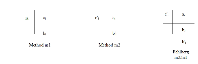
It is called Fehlberg embedded pair method with order n,m to a double method consisting in joining two Runge-Kutta methods m1, m2 with
orders n+1 and n respectively, and whose matrix A of their Butcher boards match.
We explained a little more detailed below.
Fehlberg embedded methods idea is, reached node, higher order (n+1) method is used to estimate the error
and the lowest order (n)to accept the step and move forward.
Fehlberg embedded pairs are in general known in the form METHOD_NAME_ORDER1_ORDER2.
For example, the mean New65 method uses a Runge-Kutta of order 6 to estimate
and a Runge-Kutta of order 5 to step forward.
There are other methods called Dorman-Prince wich uses the higher order method to forward and lower order method to estimate error, an example of these methods is the DOPRI54.
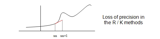
We had already talked about the Runge-Kutta methods losing precision in the case of functions with derivatives evaluated were 'bigs'.
As we will see, the Fehlber embebbed methods are a solution for this problem.
In the embedded Fehlberg pairs methods we take is two Runge-Kutta methods, m1 and m2, the first with order p+1 and the second order with order p, m1 and m2 are such that their matrix A (in the Butcher board) is the same for both.
The operation is as follows:
We take a step size h, and choose a maximum acceptable error wich we will call tolerance.
1) We calculate the solution, s1, in step with the method m1.
2) We calculate the solution, s2, in step with the method m2.
3) We take the solution provided by the method m1, s1, as the real solution.
4) We calculate the estimation as
|s1 - s2| = estimation
5a) If the estimation is minor that a certain value called tolerance, we take the solution provided by the m2 method and forward to next node by a slightly larger h.
5b)Otherwise, we reject the result, we took a step size h1 smaller than h and return to step 1
As said, the rule is: forward with the lower-order method and estimate the error with the greater order method.
It is important to note that in both cases, if the step is accepted or it be rejected, the pair embedded recalculates step size h. And it becomes smaller if the step is rejected and greater if is accepted.
How? we will see ...
These methods work well in those cases where the derivative goes through many changes because the step size changes automatically.
Fehleberg embedded pair rectifying the step size in each one of the nodes so that when the derivative is large, step forward with a smaller and on the contrary, when the derivative is small automatically increase the step size, allowing thereby saving the cost of operations.
How Fehlberg embedded pairs recalculate the step size? The answer to this question is that it depends somewhat on the method, but a general formula for an embedded pair of order n and m may be next
h' = 0.9 h min {5, (tolerance/estimation)
1/n}
Important Note: The above formula is generic, does not apply exactly to all pairs nested, although in examples tested here it had worked well.
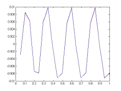
Finally, let's see an example with many changes in the derivative in the interval [0, 1], for example the problem
y' = sin100x
y(0) = - 1/100
Whose exact solution is easy to calculate is y(x) = (-1/100) cos 100x.
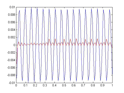
If we take the method R/K classical order 4 with 20 steps (h = 0.05) and New65f Fehlberg embedded method (this is a method which is formed with embedded pair of Runge-Kutta method of order 6 to estimate and order Runge-Kutta another 5 to forward) with 13 steps (ie an average stepsize of 0.76. If we plot the function in red and blue (repect.) those values obtained by each one of these methods, we obtain Figures the following figures:
|
|
Rk4: Note the increase of error at the points where the derivative changes, ie, at points corresponding to local maxima and minima.
|
|
|
|
New65f: Note that the graph of the function and method are indistinguishable and with 22 steps, the method is able to follow the function with only this number of steps.
|
|
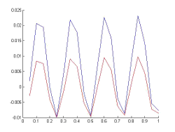
Let's take now the same problem only with the pair embedded New65f, but we are now a tolerance of 1.5 x10 -7, ie we are asking for more precision, specifically the average size step is around 0.01, we figure in color blue values obtained with the method and in color red variance step size on each node , take a look to the decreases step size for those nodes where the derivative is greater.
There are other methods in which the pair moves with higher order and estimates with the lower order (they are called methods of Dormand and Prince).