

X' (t) = f(X(t), t) ,
X(t0) = x0
Where
f: Rn x R → Rm
X: [a, b] ⊂ R → Rn
Note that this problem is really an ODEs system problem with m equations
Despite the many analytical methods to solve a Differential Equation (vector or system of equations) in real life, is greater the number of cases in which this problem can not be solved analytically, either because the solution can not be expressed in terms of elementary functions, or rather technical difficulty of finding any analytical solution.
In many cases linearizations, power series, Fourier series or infinite processes of one kind or another, are used to try to resolve the problem, at least approximately. In such cases also, solution obtained may result of small interest or unfeasible calculations on a finite but too large number of terms of any hypothetical solution.
So, numerical methods are used, mostly linear, wich compute approximate solutions on discretizations of the interval where we want these solutions were defined. The calculations are tedious, but simple computationally and easy to be programed.
For example, the problem
y' = y
y(0) = 1
We know it admits obvious solution y(x) = ex
This closes the problem, at least from a theoretical point of view. However, suppose we want to know its value and numerical value x = 10.55.
The situation is even worse if we have to integrate a function like
y(x) = ex/x
Whose solution can not be writte in elementary functions terms
Also in nonlinear equations cases, analytics solutions are very difficult to find, lets see an example: consider the case of the simple pendulum problem
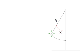
where a is the length of the rope holding the weight and x is the angle formed by rope from with vertical line.
The differential equation governing the motion of the pendulum (this equation is easily obtained from second Newton's law)
ay'' = - g sen x
where g is earth's gravity acceleration constant (aprox: g = 9.8m / s) and as stated, a is the length of the rope or bar that holds the pendulum.
this equation is usually reduced to the linear case assuming a small movement of the pendulum, at this case we can replace sin x by x. This process allows us to find an analytical solution, but it will only be approximate..
Are these cases where numerical methods are particularly useful because, for in them it is not matter equation's the linearity or nonlinearity.
